Example Forecast Data

Inspect example contrail forecast data source.

Download data

# download example data file
!wget "https://drive.usercontent.google.com/download?id=1FODPPFbTMQ2addAk2OgieYHBw92BD6dq&export=download" -O forecast.nc

--2024-10-07 17:23:51--  https://drive.usercontent.google.com/download?id=1FODPPFbTMQ2addAk2OgieYHBw92BD6dq&export=download
Resolving drive.usercontent.google.com (drive.usercontent.google.com)... 142.251.35.161
Connecting to drive.usercontent.google.com (drive.usercontent.google.com)|142.251.35.161|:443... connected.
HTTP request sent, awaiting response... 200 OK
Length: 66478078 (63M) [application/octet-stream]
Saving to: ‘forecast.nc’

forecast.nc         100%[===================>]  63.40M  15.3MB/s    in 4.4s

2024-10-07 17:24:00 (14.4 MB/s) - ‘forecast.nc’ saved [66478078/66478078]

Load in xarray

import xarray as xr

ds = xr.load_dataset("forecast.nc")
ds

<xarray.Dataset>
Dimensions:       (longitude: 1440, latitude: 641, flight_level: 18, time: 1)
Coordinates:
  * longitude     (longitude) float32 -180.0 -179.8 -179.5 ... 179.2 179.5 179.8
  * latitude      (latitude) float32 -80.0 -79.75 -79.5 ... 79.5 79.75 80.0
  * flight_level  (flight_level) int32 270 280 290 300 310 ... 410 420 430 440
  * time          (time) datetime64[ns] 2024-09-25T18:00:00
Data variables:
    contrails     (longitude, latitude, flight_level, time) float32 0.0 ... 0.0
Attributes:
    forecast_reference_time:  2024-09-25T12:00:00Z
    aircraft_class:           default
    model_version:            0.32.2

xarray.Dataset

• Dimensions:
  • longitude: 1440
  • latitude: 641
  • flight_level: 18
  • time: 1
• Coordinates: (4)
  • longitude
    (longitude)
    float32
    -180.0 -179.8 ... 179.5 179.8

    array([-180.  , -179.75, -179.5 , ...,  179.25,  179.5 ,  179.75],
          dtype=float32)

  • latitude
    (latitude)
    float32
    -80.0 -79.75 -79.5 ... 79.75 80.0

    array([-80.  , -79.75, -79.5 , ...,  79.5 ,  79.75,  80.  ], dtype=float32)

  • flight_level
    (flight_level)
    int32
    270 280 290 300 ... 410 420 430 440

    array([270, 280, 290, 300, 310, 320, 330, 340, 350, 360, 370, 380, 390, 400,
           410, 420, 430, 440], dtype=int32)

  • time
    (time)
    datetime64[ns]
    2024-09-25T18:00:00

    array(['2024-09-25T18:00:00.000000000'], dtype='datetime64[ns]')

• Data variables: (1)
  • contrails
    (longitude, latitude, flight_level, time)
    float32
    0.0 0.0 0.0 0.0 ... 0.0 0.0 0.0 0.0

    long_name :

    Contrail forcing index

    units :

    valid_min :

    0

    valid_max :

    4

    array([[[[0.        ],
             [0.        ],
             [0.        ],
             ...,
             [0.        ],
             [0.        ],
             [0.        ]],
    
            [[0.        ],
             [0.        ],
             [0.        ],
             ...,
             [0.        ],
             [0.        ],
             [0.        ]],
    
            [[0.11914641],
             [0.34592685],
             [0.65774924],
             ...,
    ...
             ...,
             [0.        ],
             [0.        ],
             [0.        ]],
    
            [[1.1190164 ],
             [1.638401  ],
             [2.6457162 ],
             ...,
             [0.        ],
             [0.        ],
             [0.        ]],
    
            [[1.2210152 ],
             [1.8187202 ],
             [2.8602548 ],
             ...,
             [0.        ],
             [0.        ],
             [0.        ]]]], dtype=float32)

• Indexes: (4)
  • longitude
    PandasIndex

    PandasIndex(Index([ -180.0, -179.75,  -179.5, -179.25,  -179.0, -178.75,  -178.5, -178.25,
            -178.0, -177.75,
           ...
             177.5,  177.75,   178.0,  178.25,   178.5,  178.75,   179.0,  179.25,
             179.5,  179.75],
          dtype='float32', name='longitude', length=1440))

  • latitude
    PandasIndex

    PandasIndex(Index([ -80.0, -79.75,  -79.5, -79.25,  -79.0, -78.75,  -78.5, -78.25,  -78.0,
           -77.75,
           ...
            77.75,   78.0,  78.25,   78.5,  78.75,   79.0,  79.25,   79.5,  79.75,
             80.0],
          dtype='float32', name='latitude', length=641))

  • flight_level
    PandasIndex

    PandasIndex(Index([270, 280, 290, 300, 310, 320, 330, 340, 350, 360, 370, 380, 390, 400,
           410, 420, 430, 440],
          dtype='int32', name='flight_level'))

  • time
    PandasIndex

    PandasIndex(DatetimeIndex(['2024-09-25 18:00:00'], dtype='datetime64[ns]', name='time', freq=None))

• Attributes: (3)

  forecast_reference_time :

  2024-09-25T12:00:00Z

  aircraft_class :

  default

  model_version :

  0.32.2

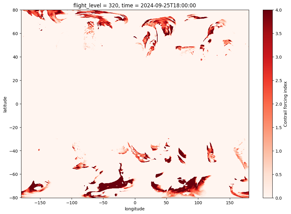
Plot continous data

# Plot continuous data at Flight Level 320 for the first timestep
ds["contrails"] \
    .isel(time=0) \
    .sel(flight_level=320) \
    .plot(x="longitude", y="latitude", cmap="Reds", figsize=(12, 8));

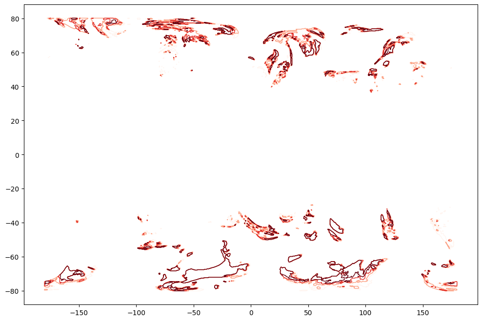
Interpret as polygons

Generate polygons for each contrail forcing index

from pycontrails.core import polygon  # pip install pycontrails

import numpy as np
from matplotlib import pyplot as plt

# Create 2D dataarray from one time and flight level
da = ds["contrails"].isel(time=0).sel(flight_level=320)

# Thresholds of interest
thresholds = [1, 2, 3, 4]

# Polygon options
longitude = da["longitude"].to_numpy()
latitude = da["latitude"].to_numpy()
min_area = 0
epsilon = 0

# Set up figure
fig, ax = plt.subplots(figsize=(12,8))
cmap = plt.get_cmap('Reds')
colors = cmap(np.linspace(0, 1, len(thresholds)))

for (c, th) in zip(colors, thresholds):

    # calculate polygons for threshold
    multipolygon = polygon.find_multipolygon(
        da.values.copy(),
        threshold=th,
        min_area=min_area,
        epsilon=epsilon,
        longitude=longitude,
        latitude=latitude,
    )

    # plot all polygons
    for poly in multipolygon.geoms:
        ax.plot(*poly.exterior.xy, color=c, lw=1)